Finite Difference Methods: Theory, Application, and Python Programming

Coming into this course, I had some prior exposure to the subject, mostly from using commercial CFD tools rather than building solvers from scratch. The finite difference treatment of 1D and 2D heat conduction connected well to problems seen in automotive battery thermal management and aerospace thermal protection analysis, even if simplified. Walking through explicit vs. implicit schemes highlighted why industry codes obsess over stability limits and time-step control. One challenge was getting boundary conditions right, especially mixed Dirichlet/Neumann cases. A small sign error at the boundary completely changed the temperature field, which mirrors real-world edge cases like contact resistance in automotive brake cooling models or insulated surfaces in aerospace panels. The beginner-level pacing was helpful, though it occasionally glossed over grid non-uniformity, which is common in production meshes. A practical takeaway was developing intuition for truncation error and stability (CFL-type limits) before trusting any plot. Coding the schemes in Python made it clear how solver choices ripple up to system-level decisions, like thermal margins or material selection. Compared with industry practice, finite volume methods dominate, but this course gave a solid foundation to understand what’s happening under the hood. I can see this being useful in long-term project work.

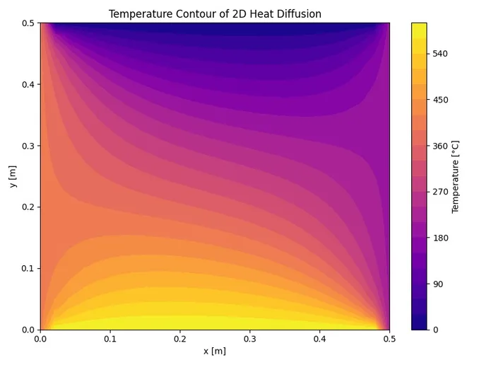
Coming into this course, I had some prior exposure to the subject. From a senior engineer’s standpoint, the material sits at a beginner level, but it still covered fundamentals that show up in real work. The treatment of the 1D heat equation mapped well to automotive thermal problems like brake rotor cooling and battery thermal management. Similar discretization issues come up in aerospace when approximating diffusion terms in preliminary CFD for wing or avionics bay heat transfer. One challenge was keeping the stability criteria straight, especially around time-step selection and CFL-like limits. That’s an area where simplified examples can hide edge cases; in production codes, violating those limits can quietly corrupt results rather than blow up. Boundary condition handling was another spot where small implementation choices had outsized effects, which mirrors what happens in industry solvers. Compared with commercial tools, the Python implementations are obviously stripped down, but that’s also the point. A practical takeaway was learning how grid spacing and time-step choices interact, and how to sanity-check results before trusting a contour plot. At a system level, that discipline matters when these models feed larger vehicle or aircraft simulations. The content felt aligned with practical engineering demands.

Initially, I wasn’t sure what to expect from this course, especially given the beginner label and how abstract finite difference methods can feel at first. The material ended up being more grounded than expected. The sections on discretizing the heat equation mapped cleanly to problems I’ve seen in automotive thermal management, like estimating temperature gradients in battery packs, and the vibration examples echoed basic aerospace structural dynamics work. One challenge was keeping track of stability limits when moving from the math to Python. It’s easy to write a solver that “runs” but quietly violates a CFL-type condition and gives misleading results. The course didn’t hide those edge cases, which was helpful, even if it meant backtracking a few times. What stood out was the emphasis on boundary conditions and grid resolution. In industry, we lean heavily on commercial FEM or CFD tools, but this course reinforced why those solvers behave the way they do, and where they can mislead at a system level. A practical takeaway was building a simple 1D transient heat solver and learning quick sanity checks before trusting the output. Overall, it felt grounded in real engineering practice.